🧲 Polar Material Analysis
This tutorial covers GPUMDkit calculator options 406-410 and the plane-grid plotting workflow.
Script Location: Scripts/calculators/ and Scripts/plt_scripts/
This tutorial includes both general and system-specific tools:
nlist,disp, andavg-structare broadly useful for structure/trajectory analysis.oct-tiltis for octahedral environments (requires 6 neighbors around each center).pol-abo3is specific toABO3polarization analysis.
Dependency
These scripts require ferrodispcalc:
Interactive mode entry
Options 406-410 are the core functions for this tutorial. The sections below explain when to use each one and how to run it.
For full argument details, use:
gpumdkit.sh -calc nlist -h
gpumdkit.sh -calc disp -h
gpumdkit.sh -calc avg-struct -h
gpumdkit.sh -calc oct-tilt -h
gpumdkit.sh -calc pol-abo3 -h
gpumdkit.sh -plt plane-grid -h
406) Build neighbor list (calc_neighbor_list.py)
Build neighbor lists for selected center and neighbor elements.
When to use it:
This is usually the first step before disp, oct-tilt, and pol-abo3, because those scripts read nl-*.dat neighbor files.
Usage
# Example 1: Ti-O nearest 6 neighbors for octahedral analysis
gpumdkit.sh -calc nlist -i model.xyz -c 4.0 -n 6 -C Ti -E O -o nl-Ti-O.dat

# Example 2: Pb/Sr-O nearest 12 neighbors for A-site centered analysis
gpumdkit.sh -calc nlist -i model.xyz -c 4.0 -n 12 -C Pb Sr -E O
Arguments (complete)
-i, --input: Input structure file. Default:model.xyz.-x, --index: Frame index to read from input. Default:0.-c, --cutoff(required): Neighbor search cutoff (Angstrom).-n, --neighbor-num(required): Number of neighbors per center.-d, --defect: Defect mode. If enabled and neighbors are insufficient, missing slots are filled with the center index.-C, --center-elements(required): Center species list.-E, --neighbor-elements(required): Neighbor species list.-o, --output: Output file path. Default:nl-<center>-<neighbor>.dat.
Output file
- Main output: neighbor list text file (for example
nl-Ti-O.dat). - The file is a 2D integer array with shape
(n_center, neighbor_num + 1). Each row corresponds to one center atom: the first column is the center index, and the remaining columns are its neighbor indices (all 1-based).
407) Calc displacement from trajectory (calc_displacement.py)
Compute local displacement vectors from a trajectory/model and a neighbor list.
Usage
# Example 1: single-frame displacement from model.xyz
gpumdkit.sh -calc disp -i model.xyz -n nl-Ti-O.dat -o disp_model.dat

# Example 2: use the last 20% frames in movie.xyz
gpumdkit.sh -calc disp -i movie.xyz -n nl-Ti-O.dat -l 0.2 -o displacements.dat
Arguments (complete)
-i, --input: Input xyz file. Default:model.xyz.-n, --neighbor-list(required): Neighbor list file fromnlist.-o, --output: Output file. Default:displacements.dat.-s, --start: Slice start index. Default:0.-t, --stop: Slice stop index. Default: end.-p, --step: Slice step. Default:1.-l, --last: Select trailing frames. Integer: lastNframes.0 < value < 1: last ratio of frames.--lastis mutually exclusive with-s/-t/-p.
Output file
- Main output:
displacements.dat(or your custom output name). - The saved text file is a 2D array: for a single-frame input, its shape is
(n_center, 3); for a multi-frame input, it is(n_selected_frame * n_center, 3)in frame-major order. The three columns aredx,dy, anddzdisplacement components in Angstrom.
408) Calc averaged structure (calc_averaged_structure.py)
Generate one averaged structure from selected trajectory frames. Use this after equilibration. For a solid near equilibrium, average a frame window at the target temperature and analyze that representative structure instead of processing every snapshot.
Usage
# Example 1: average all frames
gpumdkit.sh -calc avg-struct -i movie.xyz -o averaged_structure.xyz

# Example 2: average selected frames (100:500:2)
gpumdkit.sh -calc avg-struct -i movie.xyz -s 100 -t 500 -p 2 -o avg_slice.xyz
Arguments (complete)
-i, --input: Input trajectory file. Default:movie.xyz.-o, --output: Output structure file. Default:averaged_structure.xyz.-s, --start: Slice start index. Default:0.-t, --stop: Slice stop index. Default: end.-p, --step: Slice step. Default:1.-l, --last: Select trailing frames (last Norlast ratio).--lastis mutually exclusive with-s/-t/-p.
Output file
- Main output: averaged single-frame extxyz file.
- Position averaging applies MIC/PBC correction relative to the first selected frame.
409) Calc octahedral tilt (calc_oct_tilt.py)
Calculate octahedral tilt angles from a B-O neighbor list.
This is commonly used to analyze octahedral rotation patterns in ABO3 systems, such as SrTiO3 and PbZrO3.
Usage
# Example 1: octahedral tilt of the TiO6 octahedra from a single frame
gpumdkit.sh -calc oct-tilt -i model.xyz -n nl-Ti-O.dat -o oct_tilt_model.dat

# Example 2: octahedral tilt of the TiO6 octahedra from the last 20% trajectory frames
gpumdkit.sh -calc oct-tilt -i movie.xyz -n nl-Ti-O.dat -l 0.2 -o octahedral_tilt.dat
Arguments (complete)
-i, --input: Input xyz file. Default:model.xyz.-n, --neighbor-list(required): B-O neighbor list file.-o, --output: Output file. Default:octahedral_tilt.dat.-s, --start: Slice start index. Default:0.-t, --stop: Slice stop index. Default: end.-p, --step: Slice step. Default:1.-l, --last: Select trailing frames (last Norlast ratio).--lastis mutually exclusive with-s/-t/-p.
Output file
- Main output:
octahedral_tilt.dat(or custom name). - The saved text file is a 2D array with three columns (
theta_x,theta_y,theta_z, in degree): for a single-frame input, shape is(n_center, 3); for a multi-frame input, shape is(n_selected_frame * n_center, 3).
410) Calc polarization for ABO3 (calc_polarization_abo3.py)
Calculate local polarization vectors for ABO3 systems.
Usage
# Example 1: single-frame ABO3 polarization
gpumdkit.sh -calc pol-abo3 -i model.xyz --nl-ba nl-Ti-Pb.dat --nl-bo nl-Ti-O.dat \
  --bec Pb=2 Sr=2 Ti=4.0 O=-2.0 -o polarization_model.dat

# Example 2: trajectory polarization on a selected frame window
gpumdkit.sh -calc pol-abo3 -i movie.xyz --nl-ba nl-Ti-Pb.dat --nl-bo nl-Ti-O.dat \
  --bec Pb=2 Ti=4.0 O=-2.0 -s 200 -t 600 -p 5 -o polarization_slice.dat
Arguments (complete)
-i, --input: Input xyz file. Default:model.xyz.--nl-ba(required): B-A neighbor list.--nl-bo(required): B-O neighbor list.-o, --output: Output file. Default:polarization.dat.--bec(required): Born effective charge terms inElement=valueformat. Example:Pb=2.5 Ti=4.0 O=-2.0.-s, --start: Slice start index. Default:0.-t, --stop: Slice stop index. Default: end.-p, --step: Slice step. Default:1.-l, --last: Select trailing frames (last Norlast ratio).--lastis mutually exclusive with-s/-t/-p.
Important checks:
--becmust include all element species in the input structure.- Center atom indices in
--nl-baand--nl-bomust match.
Output file
- Main output:
polarization.dat(or custom name). - The saved text file is a 2D array with three columns (
Px,Py,Pz, inC/m^2): for a single-frame input, shape is(n_center, 3); for a multi-frame input, shape is(n_selected_frame * n_center, 3)in frame-major order. The script prints a warning if the total Born charge is not balanced.
Plane-grid visualization (plt_plane_grid.py)
You can visualize either displacements.dat or polarization.dat:
# Example 1: displacement map on Ti sites, first XY layer
gpumdkit.sh -plt plane-grid -i model.xyz -d displacements.dat -e Ti --select-xy 0

# Example 2: polarization map on Pb sites, XZ and YZ layers
gpumdkit.sh -plt plane-grid -i model.xyz -d polarization.dat -e Pb --select-xz 0 1 2 --select-yz 3 4
Arguments (complete):
-i, --input: Input xyz file for atomic layout and layering. Default:model.xyz.-d, --disp: Vector-field data file. Default:displacements.dat.-e, --elements(required): Center element symbols used to map vectors to lattice layers.-m, --tol: Layer tolerance for grid mapping. Default:1.0.-g, --target-size: Expected grid size asnx ny nz.-o, --save-dir: Figure output directory. Default:plot.-f, --frame: Frame index to visualize when vector data has multiple frames. Default:0.--select-xy: Selected XY layer indices.--select-xz: Selected XZ layer indices.--select-yz: Selected YZ layer indices.
Output:
- Creates output directory if needed.
- Saves figures as
XY_*.png,XZ_*.png,YZ_*.png.
Output files at a glance
| Script | Main output | What it stores |
|---|---|---|
calc_neighbor_list.py |
nl-*.dat |
1-based center index + neighbor indices |
calc_displacement.py |
*.dat |
Local displacement vectors (dx dy dz, Angstrom) |
calc_averaged_structure.py |
*.xyz |
One averaged structure |
calc_oct_tilt.py |
*.dat |
Octahedral tilt angles (theta_x theta_y theta_z, degree) |
calc_polarization_abo3.py |
*.dat |
Local polarization vectors (Px Py Pz, C/m^2) |
plt_plane_grid.py |
plot/*.png |
XY/XZ/YZ plane maps from vector-field data |
Real Examples
Temperature-driven Ferroelectric-to-paraelectric phase transition for PbTiO3
Assume all files are in the current directory ./:
model.xyz is the initial structure used to run MD simulations. Each TEMP K.xyz is a trajectory at that temperature.
Step 1: get averaged structures from the last half of each trajectory
for f in *K.xyz; do
  tag="${f%.xyz}"
  gpumdkit.sh -calc avg-struct -i "$f" -l 0.5 -o "${tag}-avg.xyz"
done
This writes 300K-avg.xyz, 350K-avg.xyz, ..., 800K-avg.xyz.
Step 2: build neighbor lists from model.xyz
# B-O list: for each Ti, find the nearest 6 O atoms
gpumdkit.sh -calc nlist -i model.xyz -c 4.0 -n 6 -C Ti -E O -o nl-Ti-O.dat

# A-O list: for each Pb, find the nearest 12 O atoms
gpumdkit.sh -calc nlist -i model.xyz -c 4.0 -n 12 -C Pb -E O -o nl-Pb-O.dat

# B-A list required by pol-abo3: for each Ti, find the nearest 8 Pb atoms
gpumdkit.sh -calc nlist -i model.xyz -c 5.0 -n 8 -C Ti -E Pb -o nl-Ti-Pb.dat
Step 3: compute displacement and polarization for each temperature
Use Born effective charges (BEC), not nominal ionic charges. For PbTiO3 in this example:
You can obtain BEC from your own DFPT calculation or from literature values. Thus use following commands to compute local displacement and polarization:
for f in *K.xyz; do
  tag="${f%.xyz}"
  gpumdkit.sh -calc disp -i "$f" -n nl-Ti-O.dat -l 0.5 -o "${tag}-disp.dat"
  gpumdkit.sh -calc pol-abo3 -i "$f" --nl-ba nl-Ti-Pb.dat --nl-bo nl-Ti-O.dat \
    --bec Pb=3.44 Ti=5.18 O=-2.8733333333 -l 0.5 -o "${tag}-pol.dat"
done
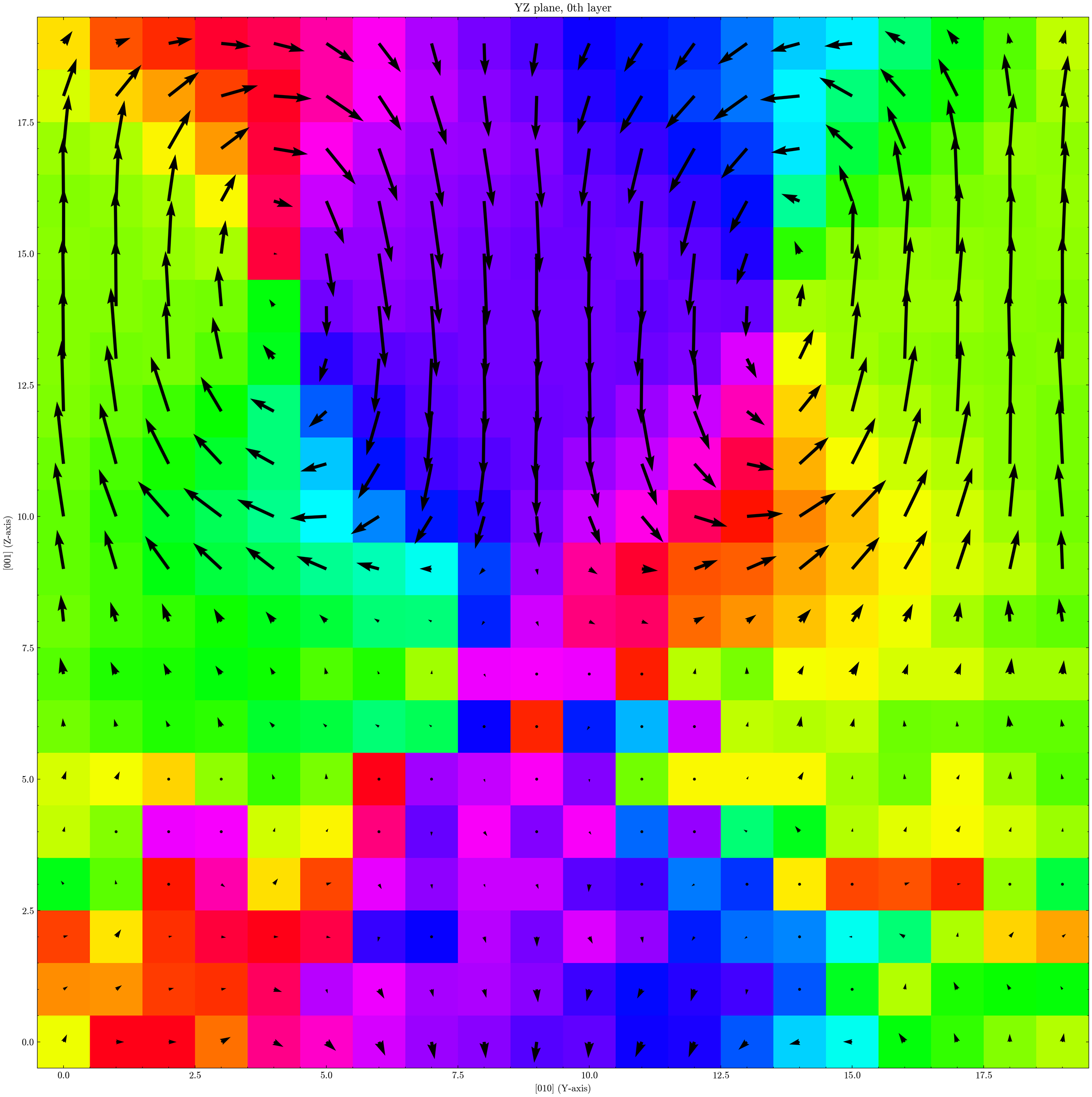
Step 4: plot displacement and polarization maps in real space
for f in *K.xyz; do
  tag="${f%.xyz}"
  gpumdkit.sh -plt plane-grid -i "${tag}-avg.xyz" -d "${tag}-disp.dat" -e Ti --select-xz 1 -o "plot-${tag}-disp"
  gpumdkit.sh -plt plane-grid -i "${tag}-avg.xyz" -d "${tag}-pol.dat" -e Ti --select-xz 1 -o "plot-${tag}-pol"
done
Step 5: build a temperature-order-parameter curve
By analyzing the lattice of each temperature-averaged structure together with its polarization (XX-pol.dat), we can obtain the following figure:
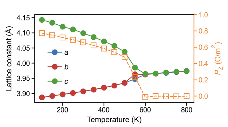
The trend shows a clear phase transition around 600 K, where the polarization vanishes.
Topological structure in PbTiO3/SrTiO3 superlattice
Assume movie.xyz is the trajectory of the PbTiO3/SrTiO3 superlattice in the current directory.
Step 1: build an averaged structure from the last 25% frames
Step 2: build the Ti neighbor list
Step 3: plot the plane-grid map
gpumdkit.sh -calc disp -i movie.xyz -n nl-Ti-O.dat -l 0.25 -o disp-last25.dat
gpumdkit.sh -plt plane-grid -i model-avg.xyz -d disp-last25.dat -e Ti --select-xy 0 -o plot-topology
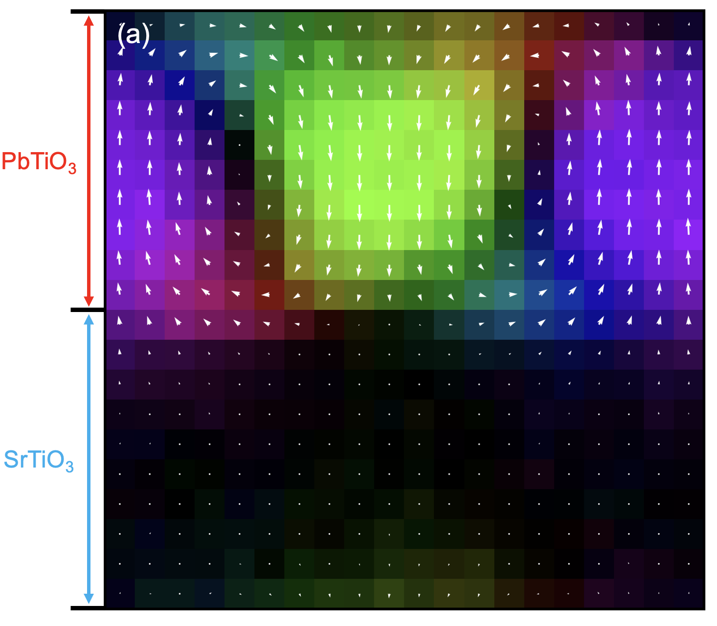
This gives a map similar to the one shown earlier. In the PTO region, a vortex-like polarization pattern is visible, while polarization in the STO region is close to zero. By analyzing how polarization varies around the vortex core, you can estimate the local dielectric response, but that is beyond the scope of this tutorial.
Note: this figure uses a different colormap from the default GPUMDkit plotting style. The default output does not look exactly the same, but you can get this style with small plotting-script changes.
Other Systems
Organic-inorganic hybrid ferroelectrics
In many organic-inorganic ferroelectrics, polarization is strongly tied to anisotropic molecular units. A practical way to track molecular orientation is to use bond vectors.
For TMCM-CdCl3, you can use the C-Cl bond direction of the TMCM molecule as an orientation proxy, then use it to estimate the polarization state:
# Find the nearest Cl around each C (tune cutoff if needed)
gpumdkit.sh -calc nlist -i model.xyz -c 3 -n 1 -C C -E Cl -o nl-C-Cl.dat

# Compute C-Cl bond vectors from the trajectory
gpumdkit.sh -calc disp -i movie.xyz -n nl-C-Cl.dat -o ccl_vectors.dat
ccl_vectors.dat can then be analyzed as an orientation order parameter. More details could be found at: Phys. Rev. Lett. 136, 016801
Other ferroelectric families
Beyond ABO3, ferrodispcalc can be adapted to many ferroelectric systems, including nitrides, hafnia-based compounds, organic-inorganic hybrids, and some 2D ferroelectrics.